Neural Network Basics for the Edge
The journey from a conceptual dataset to a functional edge device begins with a fundamental shift in perspective. Developers accustomed to the elasticity of the cloud—where compute resources are virtually infinite—must adapt to the fixed-resource reality of TinyML. In this environment, the efficiency of an algorithm is not merely measured by its accuracy, but by its Silicon Footprint and Compute-per-Watt efficiency.
This transition marks the most critical phase of the developer’s journey. While traditional machine learning frameworks allow for a degree of separation between the model and the machine, eFabric™ demands a Hardware-Aware Design philosophy. To achieve the Microwatt Scale, we strip away the overhead of general-purpose computation and move toward Silicon-Native Execution. This requires treating the model as a living part of the physical circuitry rather than a detached piece of software logic.
In the context of eFabric™, a Neural Network is not just a mathematical abstraction; it is a precisely engineered computational graph optimized for execution on silicon gates. For edge developers, understanding how layers and weights translate to hardware performance is the key to building successful products.
Layers, Neurons and Weights: A Primer
In traditional computing, logic is defined by explicit "if-then" instructions. In the eFabric™ ecosystem, logic is emergent—it is stored within the architecture of the neural network. For a developer, the network is a series of computational layers that act as a sophisticated filter, refining raw sensor data into a high-confidence classification.
The Computational Building Blocks
To build an efficient model, you must understand the three fundamental components of your network's architecture:
-
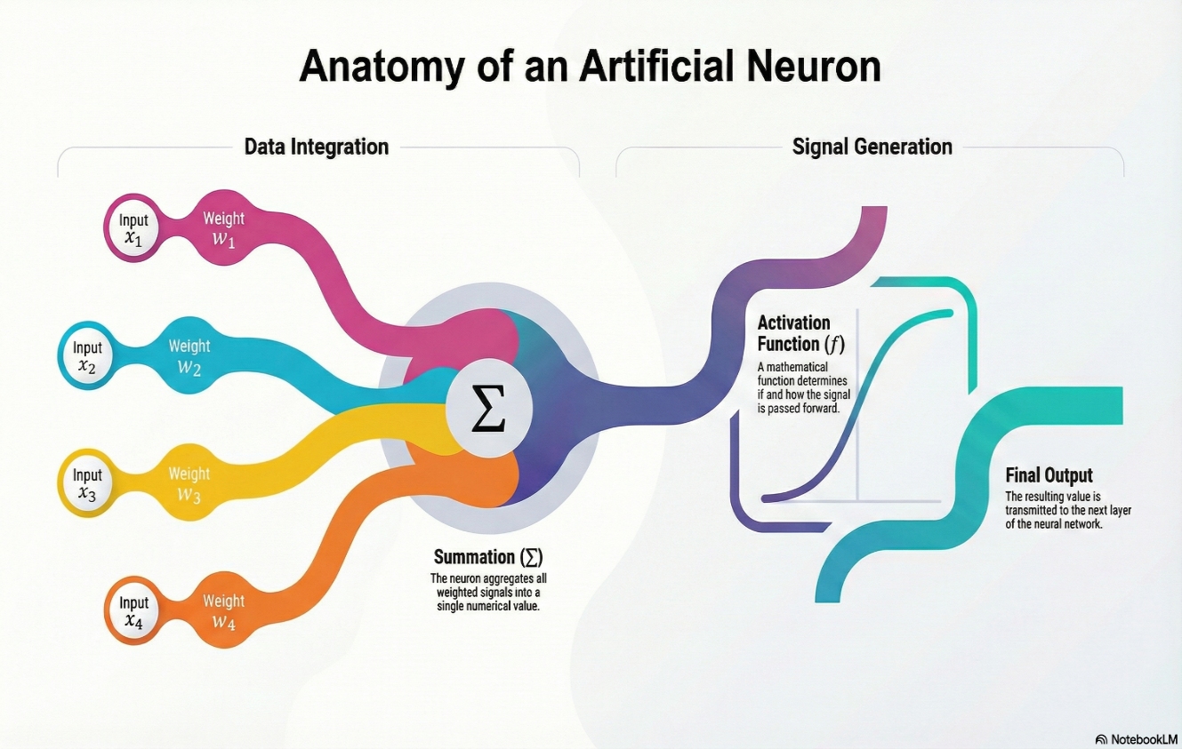
Neurons (The Processing Units): Think of a neuron as a mathematical function. It receives multiple inputs, calculates their weighted sum and applies an Activation Function (like ReLU or Sigmoid) to determine its output. In Silicon-Native Execution, these neurons are mapped to specific physical logic gates within the NDP to ensure maximum energy efficiency.
-
Weights (The Learned Memory): Weights are the core of your model's intelligence. They represent the "strength" of the connection between neurons. During the training phase in the eFabric™ Factory, the platform adjusts these weights billions of times until the network can distinguish, for example, the sound of a "security alarm" from "background chatter."
In eFabric, weights are optimized using Int8 Quantization, meaning each weight is stored as a single byte rather than a 4-byte float, drastically reducing the memory footprint.
It might not always be 8 bit. We do it for targeting Syntient current NDP series, others might have provision for 16bit, so let’s say something like depending on target hardware…>>
-
Biases (The Threshold Adjusters): A bias is an extra parameter added to the neuron's input. It allows the model to shift the activation function left or right, providing the flexibility needed to trigger a detection only when a specific "Confidence Threshold" is met.
The Layered Hierarchy
Every model created within the eFabric™ Factory is composed of layers that transform raw data into a logical decision.
-
Input Layer (The Sensory Gateway): This is where your raw digital signal enters the "Factory." This layer receives digitized signals—such as 16kHz audio PCM data or 3-axis accelerometer readings. In TinyML, the input size is strictly fixed to ensure Deterministic Inference. The Input Layer ensures the data is shaped correctly for processing.
-
Hidden Layers (Feature Extraction & Logic): This is the "Brain" of the model. These layers consist of Neurons connected by Weights.
-
Weights act as the "memory" of the network, determining the strength of the connection between neurons.
-
During training, eFabric™ fine-tunes these millions of parameters to identify specific "signatures" (e.g., the unique harmonic pattern of a siren).
eFabric uses specialized layers optimized for the Syntiant® NDP:
- Convolutional Layers (CNN): Excellent for spatial or temporal patterns (finding the "shape" of a sound).
- Fully Connected Layers: Where the high-level features are combined to form a complex understanding of the input.
-
“Model Depth vs. Power: Adding more hidden layers increases intelligence but also increases latency and power consumption. Use the eFabric Resource Estimator to find your 'Sweet Spot'.”
- Output Layer (The Decision Engine): The final destination. This layer produces a probability score. In an "Always-On" keyword model, this might be a single neuron representing the confidence level that the wake-word was heard (a single output neuron providing a value between 0 and 1, representing the probability of a match).
- Video Suggestion. Content: A 30-second animation showing a "Keyword" (like "Hey eFabric") entering the Input Layer as a waveform, lighting up specific neurons in the Hidden Layers and resulting in a "Match Found" signal at the Output Layer.
Deep Dive: The Engines of Intelligence
Convolutional Neural Networks (CNN): The Pattern Detectors
In the world of Edge AI, CNNs are the primary tool for spatial and temporal feature extraction. While often associated with image processing, in eFabric™, they are the considered standard for analyzing Spectrograms (visual representations of sound) and complex sensor patterns.
-
How it Works (The Sliding Window): A CNN uses a "filter" or "kernel" that slides across your input data. It performs a mathematical convolution to identify local patterns—such as the sharp rise in frequency of a glass break or the specific rhythmic pulse of a motor vibration.
-
Spatial Hierarchies: CNNs are structured to find simple patterns (like edges or frequencies) in the early layers and combine them into complex concepts (like a "Wake Word") in deeper layers.
-
eFabric™ Optimization: Our platform uses Depthwise Separable Convolutions where possible. This technique drastically reduces the number of parameters and computations, allowing high-performance CNNs to run within the microwatt power budget of the TML120 module.
“Use CNNs when your data has "local correlation." If the relationship between one data point and its immediate neighbor is high (like adjacent pixels or consecutive audio samples), a CNN is your most efficient choice.”
Recurrent Neural Networks (RNN): The Sequential Memory
Where CNNs excel at finding "shapes" in data, RNNs excel at understanding Time and Sequence. These are essential for "Always-on" monitoring where the context of what happened a second ago matters for the decision being made now.
-
The Feedback Loop: Unlike standard networks where data flows only forward, an RNN has a "hidden state" that acts as a memory. It feeds the output of the previous step back into the current step.
-
Gated Recurrent Units (GRU) & LSTM: eFabric™ supports advanced RNN variants like GRUs. These use "gates" to decide which information to remember and which to forget, preventing the model from being overwhelmed by background noise while waiting for a trigger event.
-
Use Case – Sequential Logic: For a Time Series Model model (e.g., a "Double Tap"), an RNN is used to ensure the model sees the sequence of Tap 1 -> Pause -> Tap 2 as a single event rather than two unrelated impacts.
Silicon-Native Mapping: CNN vs. RNN on the NDP
The Syntiant® Neural Decision Processors targeted by eFabric™ are uniquely designed to handle these architectures differently at the gate level:
| Feature | CNN Execution | RNN/GRU Execution |
|---|---|---|
| Hardware Path | Parallelized MAC (Multiply-Accumulate) units for high-speed filtering. | Dedicated feedback registers for maintaining "Temporal Memory." |
| Best For | Feature Extraction, Keyword Spotting, Image Analysis. | Sequence Modeling, Gesture Detection, Long-term Anomaly Tracking. |
| Efficiency Tip | Keep kernels small (3x3 or 1x3) to maximize Compute Density. | Use GRUs over LSTMs in eFabric™ for a 30% reduction in memory footprint with similar accuracy. |
While CNNs and RNNs provide the structural intelligence of your model, they are initially built using high-precision calculations that exceed the power budget of edge hardware. To move these "engines" from a powerful workstation to a microwatt-scale Neural Decision Processor, we must apply the science of Model Quantization.
Deep Dive: The Mathematics of Quantization
In the eFabric™ ecosystem, the most critical mathematical transformation occurs when we move a model from the high-precision world of a workstation (32-bit floating point) to the resource-constrained world of the TML120 module (8-bit integer). This process, known as Quantization, is the cornerstone of TinyML efficiency.
- What is Quantization? It is the process of "squeezing" the precision of the model from 32-bit to 8-bit.
- The Benefit: This reduces the model size by 4x and increases inference speed significantly, all while maintaining near-original accuracy.
- eFabric’s Role: Our platform performs Quantization-Aware Training (QAT), ensuring that the model "learns" to be accurate even with reduced precision, preventing the "accuracy drop" common in manual conversions.
The Linear Quantization Formula
At its simplest level, quantization is a linear mapping between a real-valued floating-point number (x) and its 8-bit integer representation (q). To achieve this, we use an Affine Mapping formula:
Where:
- q (Quantized Value): The resulting 8-bit integer (typically ranging from -128 to 127).
- x (Floating-Point Value): The original high-precision weight or activation.
- S (Scale): A positive floating-point number that "shrinks" the range of the real values.
- Z (Zero-point): An integer that ensures the real value 0.0 maps exactly to a quantized integer. This is vital for operations like Padding and ReLU activation functions.
Calculating Scale (S) and Zero-point (Z)
For every layer in your eFabric™ model, the platform must determine the optimal S and Z. This is done by analyzing the Dynamic Range [min, max] of the weights or activations:
For developers, the goal is to minimize the Quantization Error (the difference between the original and quantized value). If the dynamic range is too wide, the "resolution" of our 8-bit grid becomes too coarse, leading to a loss in model accuracy.
The Challenge: Clipping and Precision Loss
When a value x falls outside the [min, max] range of the layer, it is "clipped" to the nearest quantized boundary (q_min or q_max).
- Saturation: Too much clipping leads to a "flat" model that loses its ability to distinguish subtle features.
- Rounding Noise: The small error introduced by the round() function can accumulate across deep layers, potentially shifting the final Inference Result.
The eFabric™ Solution: Quantization-Aware Training (QAT)
While many platforms use Post-Training Quantization (PTQ)—which quantizes the model after it is already trained—eFabric™ utilizes Quantization-Aware Training (QAT).
How QAT mathematically differs:
During the training phase in the eFabric™ Factory, the platform simulates the "Int8 effects" while the model is still in its Float32 state. It introduces "Fake Quantization" nodes into the computational graph.
- The Result: The model "learns" to adjust its weights to compensate for the rounding noise and clipping errors.
- The Advantage: QAT typically recovers 98-100% of the accuracy lost during standard quantization, ensuring that your "Baby Cry" or "Wake Word" model remains robust even on ultra-low-power silicon.
[Video Suggestion: The Quantization Shift] A 60-second technical visualization showing a smooth, high-resolution wave (Float32) being overlaid by a stepped, pixelated grid (Int8). As the eFabric QAT process runs, the "pixels" shift and realign to perfectly mimic the shape of the original wave.
Supervised Learning for Pattern Recognition
In the eFabric™ ecosystem, intelligence is not programmed; it is learned. Supervised Learning is the specific machine learning paradigm we use to train models to recognize complex patterns in noisy, real-world data.
The "Teacher-Student" Model
At its core, Supervised Learning involves training a neural network using a dataset that contains both the Input Data (e.g., audio samples) and the corresponding Ground Truth Labels (e.g., "Keyword" or "Background").
- Data Labeling: For eFabric to learn, it must be "shown" thousands of examples. If you are building a Glass Break Detector, you must provide samples of actual glass breaking (Positive Samples) and samples of typical household noise like fans, TVs or speech (Negative Samples).
- Feature Mapping: The platform extracts mathematical features (like the spectrograms we discussed earlier) and maps them to these labels.
- The Objective Function: During training, the model makes a prediction. If it misidentifies a "Siren" as "Speech," the eFabric™ Factory calculates the error using a Loss Function. The weights are then adjusted via Backpropagation to minimize this error.
Pattern Recognition in Multi-Dimensional Space
For a developer, it is helpful to visualize Supervised Learning as a way to draw a "Boundary."
- The Decision Boundary: Imagine a graph where one axis is "Frequency" and another is "Duration." The neural network learns to draw a mathematical line that separates "Keyword A" from all other sounds.
- Generalization: A successful eFabric model doesn't just memorize the specific clips you uploaded; it Generalizes. It learns the essence of the pattern so that it can recognize the keyword even when spoken by a different person or in a noisy room.
“High-performance edge models require a robust set of "Background" or "Noise" data. Without a diverse set of negative samples, the model will struggle with False Positives—triggering an action when no actual event occurred.”
Inference vs. Training on the Edge
A common point of confusion for those new to TinyML is the physical location of the "learning" versus the "deciding." In the eFabric™ workflow, these two stages are strictly decoupled to maximize efficiency.
Training: The Heavy Lifting (Cloud-Side)
Training is a compute-intensive process that requires iterating over massive datasets millions of times.
- Where: This happens in the eFabric™ Cloud Factory.
- Compute: High-performance GPUs or TPUs.
- Goal: To optimize the Weights and Biases of the model through "Trial and Error" (Backpropagation).
- Output: A high-precision (Float32) trained model.
Inference: The Decision (Silicon-Side)
Inference is the "Live" phase where the trained model is deployed to the hardware to make real-time decisions.
- Where: Locally on the Syntiant® NDP (Neural Decision Processor).
- Compute: Ultra-low-power silicon gates.
- Goal: To perform a "Forward Pass"—taking new, unseen sensor data and producing a classification score in milliseconds.
- Output: A simple trigger signal (e.g., "Event Detected").
Why "Inference Only" on the Edge?
To achieve the Microwatt Scale, the TML120 module is designed for Deterministic Inference. By removing the complex "learning" circuitry from the chip, we reduce power consumption by 1000x. The chip does not "change its mind" or "learn" new things once deployed; it executes the optimized, quantized pattern it was given with absolute precision and zero latency.
The Technical Advantage: Hardware-Native Execution
Unlike generic microcontrollers that use a "software interpreter" (such as TensorFlow Lite Micro) to run a model, eFabric™ maps the neural network directly to the Silicon Logic of the NDP.
- Zero-Overhead Inference: Because the model is "baked" into the hardware's native flow, there is no CPU "searching" for the next instruction. This is the secret behind the Microwatt Scale power consumption.
- Memory Residency: In eFabric™, the entire model is designed to be Memory-Resident. It stays within the tiny on-chip RAM of the TML120 module, eliminating the high power cost of moving data to and from external memory chips.